The Oxford SWIFT Spectrograph

SWIFT Throughput and Sensitivity

SWIFT has a total efficiency (from photons above the atmosphere to detected electrons) of 23% over a large fraction of the wavelength range (see plot below). This is the same as the peak total efficiency of VLT second generation instruments (e.g. MUSE), and is at least a factor of two better than the DBSP spectrograph at the 200 inch.

Measured Throughput

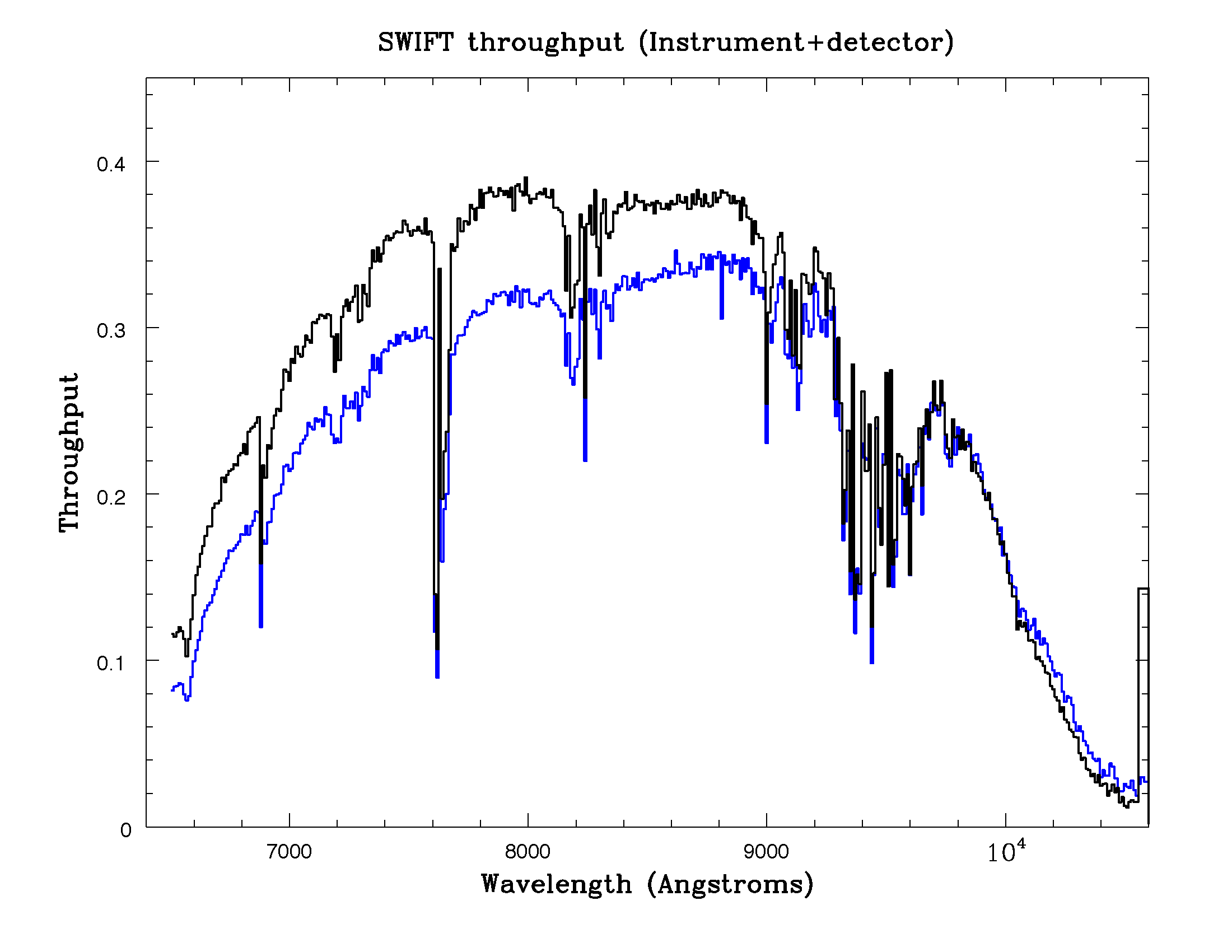
The plot below shows the measured throughput of the instrument, including the detector. The assumed throughput for the telescope and the AO system is 0.75 and 0.8 respectively. The black curve is for the master chip (science grade detector), the blue curve is for the slave chip (engineering grade detector). Note that the sensitivity stays high at very long wavelengths, up to 1 micrometer. Beyond 9000 Angstroms, SWIFT is at least twice (and probably thrice) as sensitive as a typical observatory spectrograph with a standard CCD detector array. Note that the atmospheric transmission profile has not been removed from the throughput plot.

Expected sensitivity

IFS sensitivity computations can be quite complex, as one has to consider both the spatial and spectral properties of the source. For point sources, a substantial gain in sensitivity can be had by combining the flux for all spaxels (spatial pixels), each of which contain the same spectral information. In photon noise dominated situations (either from source or sky background) the gain is typically √N, where N is the number of spaxels over which the point source light is spread out.

On the other hand, for very extended sources, the sensitivity can appear to be rather poor, but it should be kept in mind that the quoted numbers are often per spatial and spectral pixel, whereas, typically, one is only interested in information on spatial scales at least as large as the PSF (seeing or AO), and often larger (dictated by source characteristics). In both cases, substantial sensitivity gains are achieved by summing over all spaxels within the extraction aperture (typical gain √N, where N is the number of spaxels that are summed over).

The following tables list the expected sensitivity of the instrument, and the assumptions that underlie these computations. An Exposure Time Calculator (ETC) is under development, and will be available on these web pages soon. The plot at the bottom shows the measured throughput for the spectrograph, using observations of a spectrophotometric standard taken in May 2009.

The following input parameters have been used to estimate the expected line and continuum sensitivity of the instrument. An exposure time calculator will shortly be available for detailed sensitivity calculations. In the meantime, expected performance can be scaled using the two examples provided below.

• Detector read noise: 3.2/4.1e^- per pixel for the two readouts of the master chip, and 4.3/4.1e^- per pixel for the slave chip.
• Detector dark current: 8e^- per hr per pixel.
• Detector gain: 0.97 and 1.04 e^-/ADU for the master and slave chips respectively.
• Instrument throughput: The most realistic estimate of the instrument throughput (excluding telescope, AO and detector) is given by the following table.
  
  

  SWIFT instrument throughput

  Wavelength (nm)	650	700	750	800	850	900	950	1000
  Transmission	31.9%	38.1%	46.2%	50.6%	49.7%	48.0%	42.0%	29.5%

  
  
• Detector Quantum Efficiency: The LBNL thick (250 μm), fully-depleted CCD arrays provide unsurpassed QE at long wavelengths, providing SWIFT with a sensitivity gain of over a factor of three at long wavelengths, compared to normal CCDs. The detector QE at the operating temperature of 140K is given as
  
  

  SWIFT detector Quantum Efficiency

  Wavelength (nm)	650	700	750	800	850	900	950	1000
  Q.E.	0.87	0.88	0.9	0.92	0.92	0.92	0.83	0.45

  
  
• Telescope optics throughput: 0.75 (two Al reflections at 0.875 each)
• AO system science throughput: 0.8 (6 reflections at 0.98 (freshly recoated optics), plus one dichroic beamsplitter at 0.9)
• AO ensquared energy gain: factor of 1.6 gain in ensquared energy in the central pixel due to sharper core, no gain if extraction aperture is ≈ seeing disk size.
• Atmospheric transmission: assumed to be unity (detailed atmospheric transmission curve will be implemented in the ETC)
• Night sky background (average lunar illumination conditions): I band 19.5 mag ⁄arcsec², z band 18.3 mag ⁄arcsec²
• Detector exposure times (DIT): 30 minutes (1800 secs) per exposure, longer exposures are made up of NDIT sub-units DIT seconds long.
• Expected continuum sensitivity: For a z = 22 mag (Vega) point source, we obtain an SNR of 1.5 in the continuum (per spectral pixel) in a single 30 min exposure, in 1″ seeing.
• Expected line sensitivity: For a source with a line flux of 1e-17 ergs s^-1 cm^-2 arcsec^-2, with a line width of 150 km s^-1, we obtain an SNR of 1 in the line a single 30 min exposure per spatial pixel. This corresponds to an SNR of 4 per 1″ extraction aperture in the same time.